When Do Causal ML Models Beat LM / GLM / GBM? | R-bloggers

[This article was first published on blog_philipppro, and kindly contributed to R-bloggers]. (You can report issue about the content on this page here) Want to share your content on R-bloggers? click here if you have a blog, or here if you don't. Summary Who this is for: Data scientists and analysts who need to estimate what an intervention does (a call, a discount, a campaign) and want to know when causal ML methods are worth using over LM, GLM, and GBM. The basis is nine simulations with a known true effect, each with 40 repetitions. The five most important findings Data first, algorithm second.

If the model contains a wrong variable or omits an important influencing factor, all methods are equally wrong, including the most flexible ones. Only domain knowledge or an instrument helps here (Cases 4, 5). For the average effect, causal ML wins only when influencing factors act nonlinearly.

In that case the LM is clearly biased and Double ML is almost right. The difference comes from the construction principle (first adjust, then estimate), not from a particular algorithm (Case 3). A risk model is not an effect model.

Calling the customers with the highest cancellation risk achieves less than a random selection, because precisely these customers are hardly retainable any more (Case 7). The correct ranking is easier than the correct magnitude. A simple GLM can select the right units and still misstate the size of the effect (Case 9).

The causal forest pays off when the size of the effect per unit matters and its form is unknown (Cases 8, 9). In simple worlds, a well-specified GLM is better (Case 6). How to read this report?

Choose a method: Guide (next section), with two decision trees and a table. Understand the methods: Methodology, with terms, formulas, strengths and weaknesses, and the question of how to check without a known effect. Verify the evidence: Simulation, with nine cases, each with data, results, and a lesson.

The numbers [n] in the text refer to the references at the end. Guide: Which Method When? Work through the steps from top to bottom.

Stop at the first point where the answer is “not possible”: no algorithm decides steps 1–3; only step 4 chooses the method. “Unit” stands for anything that is treated (customer, person, contract, branch); the examples in the cases are set at a fictional online fitness subscription service (an app with training plans and classes). The terms used in the guide: A/B test: Who is treated was determined at random (technical term: randomized). Treated and untreated units are therefore comparable.

No random assignment (called “non-random” for short in the table): The treatment followed rules or judgments; the data simply accumulated (technical term: observational data). Treated and untreated units already differ beforehand. Influencing variable (confounder): A variable that influences who is treated and the outcome.

Measured means it is in the data. Not measured: It is missing, and no algorithm can replace it. Instrument: A random nudge that shifts the treatment but affects the outcome only through it (e.g. a randomly sent invitation).

Allows an estimate even though a confounder is missing. Average: A single effect for all units together (technical term: ATE). Answer to “Does the intervention work on average?”.

Ranking (targeting): Deciding whom to treat, e.g. the 30% with the largest effect. Only who comes first matters; a model may over- or underestimate the effect by the same amount for everyone. Effect per unit (CATE): The exact size of the effect for each unit, e.g. to weigh costs and benefits per unit.

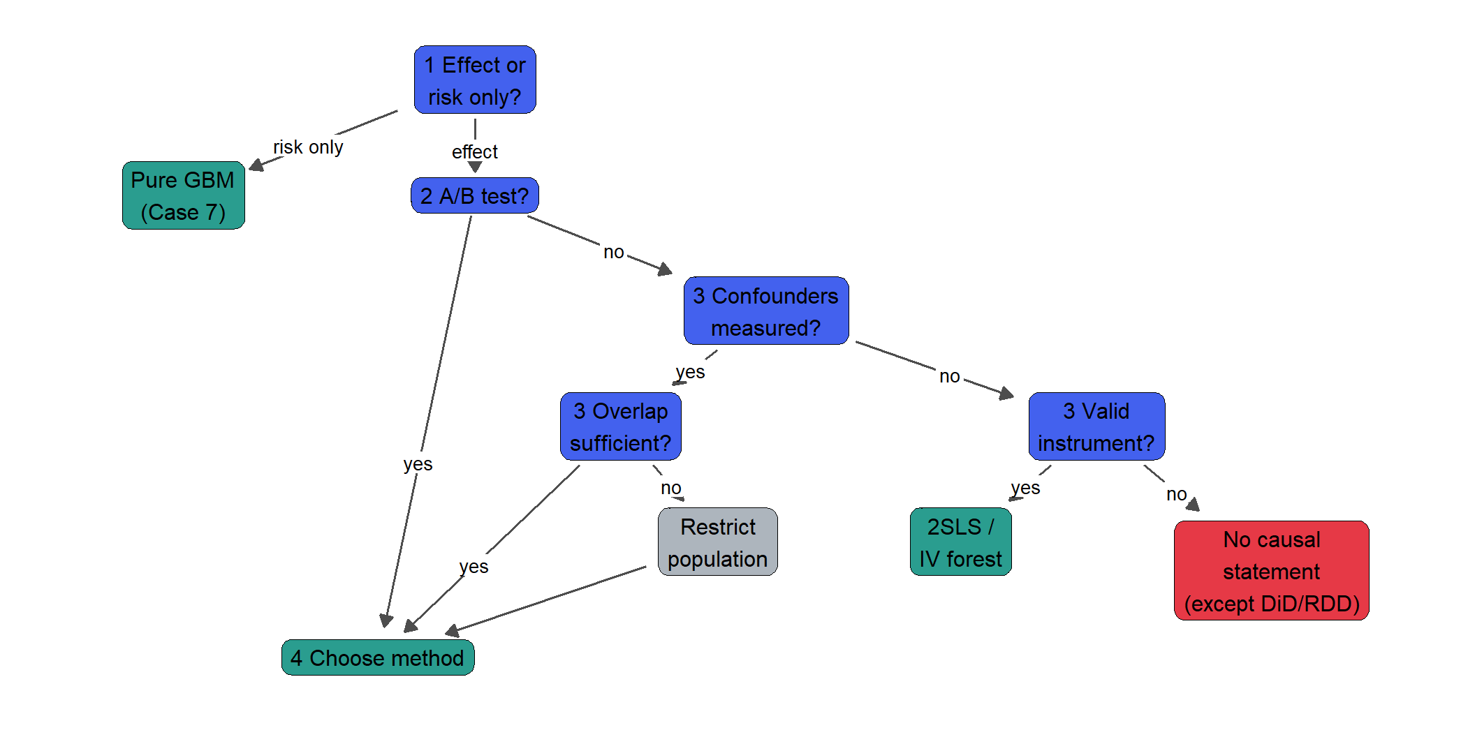
Stricter than the ranking: A model can rank correctly and still estimate the size wrongly (Case 9). Blue = question, green = recommendation, red = stop. Step 1 – What is the decision?

Question Target quantity Next Does the intervention work on average? Average (ATE) Step 2 Whom should I treat? Ranking of units by effect Step 2 How large is the effect for this unit? (e.g. for cost-benefit per unit) Effect per unit (CATE) Step 2 Who will cancel? (without intervention) Risk, no effect Pure GBM, done.

Unsuitable for decisions about interventions (Case 7: top-30% uplift 0.037, worse than chance). How strongly should I treat? (e.g. discount level) Dose-response curve Methodological knowledge, not simulated (see conclusion, continuous treatment). Step 2 – How was the treatment assigned?

At random (A/B test, lottery): Identification is secured, continue with step 4. By rules or by judgment of the business department (no random assignment): continue with step 3. Randomly assigned, but not everyone received the treatment (e.g. call assigned, customer not reached): The comparison of means by assignment measures the effect of the assignment.

For the effect of the treatment itself, the assignment serves as an instrument (2SLS, Case 5 [5]). Not simulated. Step 3 – Identification (only without random assignment) This is where most projects fail, and no algorithm helps.

Three terms decide which variables belong in the model. They differ only in where the variable sits in the cause-and-effect picture ( = treatment, = outcome, = the variable in question): Term Structure What is it? Example In the model?

Confounder \(T \leftarrow X \rightarrow Y\) A common cause: \(X\) influences who is treated and the outcome. Treated and untreated units therefore already differ before the treatment. Age: Older customers are more likely to receive a call and, for their own reasons, cancel more or less often.

Yes. Otherwise the influence of \(X\) is read as an effect of \(T\) (bias). For nonlinear influence, also in the right form (Case 2, 3).

Mediator \(T \rightarrow X \rightarrow Y\) An intermediate station: \(T\) acts on \(Y\) through \(X\). \(X\) only arises after the treatment and carries part of the effect. Call \(\rightarrow\) customer sets up a training plan \(\rightarrow\) stays. “Training plan set up” is the mediator. No, if the total effect is of interest.

Otherwise the part that runs through \(X\) is missing (Case 4). Collider \(T \rightarrow X \leftarrow Y\) A common consequence: \(X\) is influenced by \(T\) and by \(Y\). \(X\) arises after both. Call and cancellation both lead to the customer ending up in the complaint log. “In the complaint log” is the collider. No. Otherwise a spurious relationship between \(T\) and \(Y\) arises.

Not simulated as a separate case; same rule as for the mediator. Rule of thumb: What exists before the treatment and co-determines it belongs in the model. What arises after the treatment does not.

Whether a variable is a confounder or a mediator is not revealed by the data – it is domain knowledge about the process. Which variables go into the model? What exists before the treatment and co-determines it goes in (confounder).

What arises after the treatment stays out (mediator, collider). The data do not say which is which; this is domain knowledge. In Case 4 all algorithms are equally biased when the mediator is included.

Overview of good and bad control variables: [19]. Tool: Draw the process as a DAG in DAGitty; the program names the required variables [26]. Is a confounder missing?

Cannot be proven from the data. Hints come from the placebo test (an outcome that the treatment cannot influence must show effect 0; Case 5) and the E-value (how strong a missing confounder would have to be to explain away the effect) [20]. DoWhy runs such tests automatically [27].

If one is missing, is there an instrument? A random nudge that acts only through the treatment. Yes: 2SLS for a constant effect, Instrumental forest for a varying effect (Case 5).

Validity cannot be checked from the data. No: no causal statement. Label the number as an association, not as an effect.

Exception: If before-after data or a threshold exist, see difference-in-differences and regression discontinuity under “Further methods (not simulated)”. Overlap: Are there treated and untreated units in every group? Check with the propensity histogram (section “Overlap diagnostic”).

Propensities near 0 or 1: restrict the population to the region with overlap. AIPW and other weighting estimators otherwise become unstable (Case 3, †). The restriction itself is not simulated here.

Step 4 – Choose a method First find the data situation (column 2) and the question (column 3); the terms are defined at the beginning of the guide. As a decision tree, from top to bottom (blue = question, green = recommendation, red = stop; Var. = variables). It presupposes that step 3 is passed (including overlap) and that the question concerns an effect, not pure risk.

With little data (a few hundred units), row 2 of the table applies. The table additionally lists a cross-check and what to avoid: # Data situation Question Recommendation Cross-check Avoid Evidence 1 A/B test Average Comparison of means. LM (T + X) at most for variance reduction. – – Case 1, 6–8 2 A/B test, little data (a few hundred) Ranking or effect per unit First check whether the effect varies at all.

Without a strong prior hypothesis, use the average for everyone (LM T + X, CATE-RMSE 0.141 in Case 1). Causal forest (0.21): estimates an almost constant effect when the effect is constant T-learner and GBM S-learner (CATE-RMSE 0.72 and 0.51, respectively): invent differences from noise Case 1 3 A/B test, few variables, simple form plausible Ranking or effect per unit GLM with T x X (CATE-RMSE 0.127 vs. causal forest 0.24). S-learner, causal forest Pure risk model (Case 7) Case 6, 7 4 A/B test, many variables, form unknown Ranking S-learner (top-30% uplift 1.64 vs. oracle 1.65).

Causal forest, R-learner (equally good selection) Double ML and AIPW (only deliver an average), pure risk model Case 8 5 A/B test, many variables, form unknown Effect per unit Causal forest (CATE-RMSE 0.28 vs. S-learner 0.45). Also provides confidence intervals. R-learner (0.36) GLM with T x X (0.74) or with all 2-way interactions (1.08) Case 8 6 No randomization; confounders measured, linear Average LM (T + X).

Double ML Naive comparison Case 2 7 No randomization; confounders measured, nonlinear or unknown Average Double ML with a GBM as building block. AIPW, causal forest LM and S-learner (biased) Case 3 8 No randomization; confounders measured Ranking R- or S-learner (top-30% uplift 2.70 and 2.71, respectively, vs. oracle 2.74). Causal forest Pure risk model Case 9 9 No randomization; confounders measured Effect per unit Causal forest (ATE bias -0.020, CATE-RMSE 0.26).

R-learner (0.34) LM/GLM (ATE bias -1.76: ranks correctly, size wrong). AIPW: no result in 21 of 40 runs. Case 9 10 No randomization; confounder missing, instrument available Average 2SLS (constant effect) or Instrumental forest (varying effect).

Placebo test (Case 5) All methods without an instrument Case 5 11 No randomization; confounder missing, no instrument Any question about the effect No causal method. Report the association, E-value as sensitivity analysis. Exception: With before-after data or a threshold, difference-in-differences or regression discontinuity are possible (not simulated). – Any method that outputs an effect number Case 5 Step 5 – Check without knowing the truth A/B test: Qini/uplift curve and calibration on a hold-out dataset are valid.

No random assignment: R-loss ranks the methods only as long as step 3 holds. In addition, placebo test and overlap histogram. Agreement of several methods proves nothing: In Cases 4 and 5 all methods agree and are wrong.

State the uncertainty: An estimate should come with a confidence interval (Methodology, “Confidence intervals”). It measures only the random error: If step 3 is violated, even a narrow interval misses the target. Details in the section “Evaluation without knowing the truth”.

Step 6 – When in doubt Keep the simplest correct model as the baseline. Adopt the more complex method only if it is clearly better on validated data. In Cases 1, 2 and 6, complexity brings nothing.

Not tested (statements about these are methodological knowledge, not simulation): more than 100 variables with weak heterogeneity, trimming under weak overlap, weak instrument, incomplete compliance, panel/time structures, multiple treatment levels, continuous treatment, and the methods in the section “Further methods (not simulated)” (e.g. BART, BCF, TMLE). Other decision aids A fully automatic decision tree that chooses the right method from the data alone does not exist, and cannot exist: Whether a variable is a confounder or a mediator is not in the data (Case 4). Any automation therefore needs a cause-and-effect picture (DAG) based on domain knowledge as input.

What does exist: DAGitty [26]: You draw the DAG; the program names the variables that must go into the model, and possible instruments. Automates step 3.1. DoWhy [27]: From the DAG through identification and estimation to automatic checks (placebo, random additional confounder, subsamples).

Closest to an automatic workflow. EconML Library Flow Chart [28]: Decision tree for choosing the estimator, similar to the one in step 4. Additionally asks about compliance and whether the effect depends linearly on the features.

Causal Roadmap [24] and Target Trial Emulation [25]: standardized workflows from epidemiology. You first describe the experiment you would have liked to run, and then check how close the data come to it. Automatic model selection for CATE (e.g. causaltune based on EconML): chooses the estimator via R-loss or similar measures.

This works only if identification holds (see “Evaluation without knowing the truth”). Methodology This part describes what is estimated and with which methods, without simulation results: the core idea, the terms, the methods studied with their formulas, and the question of how to check a method on real data (where the true effect is unknown). Core idea LM, GLM, and GBM are normally trained to predict Y.

CausalML models are built to estimate the effect of a treatment T on Y, either on average (ATE) or per unit (CATE). A good prediction model is not automatically a good effect model. Conversely, an effect model is not automatically better when the world is simple.

In real data the true effect is never known. That is why we simulate here: we define the formulas that generate the data ourselves. We therefore know the true effect of every single unit and can measure each method against it exactly.

Classification following Molnar [6]: the report takes the causal inference mindset (what causes what?) and uses supervised learning (prediction models such as GBM) only as a building block, e.g. in Double ML. Evaluation is frequentist (bias and spread over repeated samples). Other mindsets lead to other tools: Bayesian to BART and Bayesian causal forest (uncertainty per unit as a posterior), reinforcement learning to bandits, which assign the treatment continuously and learn while doing so.

That is a different type of data than the one used here. The core message in this language: a good supervised-learning model is not automatically a good causal-inference model. Introductions to the field: [1, 2, 3].

Terms Potential outcomes. Every unit has two possible outcomes: if it is treated () and if not (). Only one of them is ever observed.

The individual effect is . Term Definition ATE (Average Treatment Effect) \(\text{ATE} = E[Y(1) – Y(0)]\): effect on average across all units. CATE (Conditional ATE) \(\tau(x) = E[Y(1) – Y(0) \mid X = x]\): effect for units with characteristics \(x\).

This is the effect “per unit”. Treatment \(T\) The action whose effect we are interested in (call, discount, campaign). Always 0/1 here.

Outcome \(Y\) The outcome the action is supposed to influence. Higher = better. Confounder Variable that influences both T and Y (\(T \leftarrow X \rightarrow Y\)).

If it is ignored, the comparison of treated vs. untreated mixes the effect of T with the effect of X. Must be in the model, and in the correct functional form. Mediator Variable on the path from T to Y (\(T \rightarrow M \rightarrow Y\)); it arises after T.

Adjusting for it removes the part of the effect that runs through M. Must not be in the model if the total effect is of interest. Collider Variable that is influenced by T and Y (\(T \rightarrow C \leftarrow Y\)). Adjusting for it creates a spurious relationship between T and Y.

Must not be in the model. (Not a separate case here; same rule as for the mediator: nothing that arises after T.) Instrument \(Z\) Variable that influences T but affects Y only through T (\(Z \rightarrow T \rightarrow Y\)) and is unrelated to unobserved disturbances. Allows effect estimation despite unobserved confounding. Effect modifier Variable on which the size of the effect depends (e.g. the discount only works for price-sensitive customers).

Creates heterogeneity: \(\tau(x)\) is not constant. Noise variable Variable with no influence on T or Y. Does not harm systematically, but costs estimation precision.

Randomization T is assigned by chance (coin flip). Then there are no confounders for T, and the simple comparison of means is unbiased. In the diagrams (DAGs) below, an arrow means: “A enters the formula of B”.

Dashed = unobserved variable. Methods All methods receive the training data as input and return an estimated effect for every test customer as output. Exception: the “pure” GBM, which ignores T and only predicts a risk.

Method Model Assumption Naive (diff. in means) \(\hat\tau = \bar Y_{T=1} – \bar Y_{T=0}\) No confounding (randomization) LM/GLM (T + X) \(Y = \beta_0 + \tau T + \beta^\top X\) Effect constant; Y linear in X (logit-linear for binary Y) LM/GLM (T x X) \(Y = \beta_0 + \tau_0 T + \beta^\top X + T \cdot \gamma^\top X\) Effect linear in X LM/GLM (T x all 2-way X) like T x X, plus all products \(X_j X_k\) and their interaction with T Effect quadratic in X GBM / LightGBM S-learner \(\hat f(X, T)\) = one GBM with T as a feature; \(\hat\tau(x) = \hat f(x, 1) – \hat f(x, 0)\) No form imposed. Regularization can push the effect of T toward 0. GBM / LightGBM T-learner \(\hat f_1\) on treated, \(\hat f_0\) on untreated; \(\hat\tau(x) = \hat f_1(x) – \hat f_0(x)\) No form imposed.

Two separate models, each with half the data: high variance. GBM / LightGBM pure (ignores T) \(\hat f(X)\) without T; score = predicted risk \(-\hat f(x)\) No effect model. This is how targeting is often done (churn model, then call the highest-risk units).

Causal forest grf::causal_forest No form imposed. Estimates \(\tau(x)\) directly, adjusted for propensity and baseline (honest trees). Default settings.

ATE here = mean of the CATE predictions. Double ML (xgboost) Cross-fitting (5 folds): \(\hat\ell(X) \approx E[Y \mid X]\), \(\hat m(X) \approx E[T \mid X]\) via xgboost; \(\hat\tau = \frac{\sum_i (T_i – \hat m_i)(Y_i – \hat\ell_i)}{\sum_i (T_i – \hat m_i)^2}\) Effect constant (or weighted mean); confounders arbitrarily nonlinear. Same xgboost as the S-learner, but T and Y are first residualized on X, so regularization does not bias the effect.

R-learner (xgboost) Same residuals \(\tilde Y, \tilde T\) as Double ML; \(\hat\tau(x)\) = xgboost on \(\tilde Y / \tilde T\) with weights \(\tilde T^2\) No form imposed for \(\tau(x)\); confounders arbitrarily nonlinear. Double ML with a varying effect. Needs overlap: units with propensity near 0/1 contribute little.

AIPW (causal forest) grf::average_treatment_effect on the causal forest: \(\hat\tau = \tfrac{1}{n}\sum_i \big[\hat\mu_1 – \hat\mu_0 + \tfrac{T_i (Y_i – \hat\mu_1)}{\hat e} – \tfrac{(1-T_i)(Y_i – \hat\mu_0)}{1 – \hat e}\big]\) Doubly robust: correct if the outcome model or the propensity model is correct. Average effect only, no effect per unit. 2SLS Stage 1: \(\hat T\) = prediction from \(T \sim Z + X\) Stage 2: \(Y = \beta_0 + \tau \hat T + \beta^\top X\) Valid instrument Z; effect constant.

Classical IV estimator. Instrumental forest grf::instrumental_forest Valid instrument Z; effect may depend arbitrarily on X. xgboost and LightGBM: depth 3, learning ra